
Butterfield 1
Murder Rates and the Death Penalty: A Post-Moratorium Era
Brian Butterfield
University of Akron
Department of Economics
Senior Project
Spring 2020

Butterfield 2
Acknowledgement
I would like to thank the entire Economics department for what I have learned during my
collegiate career. To specifically mention Dr. Renna, without whose dedication I would not have
made it through this senior research project. Additionally, Dr. Erickson’s constant feedback on
drafts helped keep me motivated. In an unprecedented time to be a graduating senior, her
telephone advice gave me the confidence to cross the finish line.
Thank you.

Butterfield 3
Abstract:
This paper intends to build upon the limited research in recent years that has
been conducted on the criminal significance of the death penalty. I pose to determine if
there is a significant deterrent effect of murder through the use of the death penalty in the
United States in a moratorium era. Given the controversy of the results of past studies, I
find that higher execution rates have a slight impact in raising the US murder rates. A 1
percent increase in execution rates increases murder rates by a slim 0.01 percent via
OLS. With using the panel data in a one-way fixed effects, the significance strengthens to
a 0.082 percent increase in murders for every 1 percent increase in executions.

Butterfield 4
Table of Contents
I. Introduction 5
II. Survey of Literature 8
III. Theoretical Model Development 11
IV. Model Specification and Results 14
V. Results Interpretation 17
VI. Conclusion 19
VII. References 22
VIII. Appendix 24
IX. SAS Code 27

Butterfield 5
I. Introduction
The Death Penalty Information Center reports that more than 165 individuals wrongly
accused of violent crimes have been executed in the United States since 1973. This does not
include others who had claimed their innocence. The death penalty is as controversial as gun
rights and abortion laws; even before the signing of the Declaration of Independence, there were
arguments for and against capital punishment in the colonies. As of 2020, the American divide is
greater than ever, with 30 states using the death penalty as legal recourse.
Much of the debate stems from the standpoint of morality. Supporters believe capital
punishment is a fitting penalty for the severity of the crime, and taxpayers should not be required
to support a murderer’s life sentence in prison. In contrast, opponents often object on the basis of
moral and religious principle. Some support the death penalty because they believe it prevents
crimes from being commmitted, while others disagree.

Butterfield 6
Figure 1: The comparison of murder rates between death penalty states and non-death penalty states (per 100,000 residents), per the
1
Death Penalty Information Center
According to the Death Penalty Information Center, (Figure 1) over the past 28 years,
states with the death penalty have a higher murder rate per 100,000 residents on average
compared to states that do not have capital punishment. The motivation for the research is not to
determine if there is a significant statistical connection nor a correlation between murder rates
and executions, although there is in fact a conflict in that research itself. The purpose is to
determine if there is a deterrent, and to what effect
. The economic motivation is twofold.
1
https://deathpenaltyinfo.org/facts-and-research/murder-rates/murder-rate-of-death-penalty-states-compar
ed-to-non-death-penalty-states

Butterfield 7
It is important to note that from an economic perspective, the marginal benefits and
marginal costs are the most meaningful when studying allocative efficiency. The additional
benefits of the death penalty are those associated with life imprisonment. That is, the marginal
benefits are the difference between the total benefits of the death penalty and the total benefits of
life imprisonment. Many analyses produce monetary estimates of the cost to put one to death.
However, these studies produce total cost estimates, not marginal cost estimates. From an
economic perspective, society should only use capital punishment if the marginal benefits
outweigh the marginal costs. In the course of analyzing the economic efficiency of capital
punishment, and before providing any recommendations, both the benefits and costs of the death
penalty must be evaluated. Many innocent men die on death row, further creating rifts between
races and classes. The second economic motivation is to reduce murder in the United States,
where murder always negatively affects the economy and welfare of a society. Although this
study does not look at costs versus benefits of the death penalty specifically, it can lead to a
conversation about the viability of the punishment with more data given.
Capital punishment is again a highly debated topic in the United States because of the
moratorium of the death penalty. In a newfound era of controversy of the death penalty, with an
additional ten states at the turn of the century at least considered its moratorium, (Dezhbakhsh)
new evidence is needed on the effectivity of the punishment. Further study into the
post-moratorium states can help strengthen or weaken both sides of the arguments.
The Research Question

Butterfield 8
The aim of this study is to analyze the effectiveness of the death penalty as a murder
deterrent in a post-moratorium era in the United States, and whether it has changed from earlier
periods.
II. Survey of Literature
The fundamental basis of the link between crime and economics is derived from Gary
Becker’s economic theory of crime (1968). The theoretical framework applies simple economic
principles of consumer behavior in a market in which people choose to commit crimes. Becker
established that crime is committed on the basis of rationality, cost to benefit analysis of the
potential offender, and utility maximization. However, this analysis only pertains to rational
decision makers that commit a non-violent crime. Many studies used Becker’s theory to expand
on situations in which the perpetrator commits a violent crime, with assault, rape, and murders
being the forefront area of study. As a result, this original theory lead to the breakdown analysis
of murder versus capital punishment.
Building upon Becker’s original theory, numerous econometric studies have been
conducted to examine the effect of the death penalty as a murder deterrent. Most of the studies
use time series and panel data to measure the effect. Isaac Ehrlich’s (1975) research was one of
the original pioneering studies on whether execution rates cause a decrease in murder rates in the
United States. By extending Becker’s theory of the rational offender, Ehrlich developed a
positive approach towards testing the deterrence hypothesis using multiple regression techniques.
The study used U.S. aggregate time series data over a 35 year period as its structure, and
suggested a significant deterrent effect, sharply contrasting with earlier findings. Critics of

Butterfield 9
Ehrlich later addressed the issue of his findings: the proper functional form of the relationship
between the murder rate and its determinants. It is claimed that evidence of a deterrent effect is
found within the logarithmic form but not with the linear form, and therefore Ehrlich’s results
depended entirely on his choice of functional form.
Ehrlich inspired an interest in econometric analysis of deterrence, leading to many studies
that used his data, but included different regressors or different choices of endogenous vs.
exogenous variables. As a consequence, economists have argued against the viability of
researching the death penalty’s implication on homicide rates. Katz (2003) argued that the
quality of life in prison is likely to have a greater impact on criminal behavior than the death
penalty. Using state-level panel data covering the period 1950-1990, he demonstrated that the
death rate among prisoners (due to prison conditions) is negatively correlated with crime rates,
consistent with deterrence, and with robust findings. Furthermore, it was found that there is little
systematic evidence that the execution rate influenced crime rates in that time period.
Dezhbakhsh (2003) focused on post-moratorium panel data of the effect of the death
penalty as a murder deterrent. They examined the deterrent hypothesis using county-level,
post-moratorium panel data and a system of simultaneous equations. The procedure employed
overcame common aggregation problems using panel data from 1977-1996. It eliminated the
bias arising from unobserved heterogeneity, and provided evidence relevant for current
conditions, such as the current crime situation in the model. As a result, the findings suggested
that capital punishment has a strong deterrent effect, similiar to Ehrlich’s findings.
Introducing a panel study of United States state-level data over a twenty year period,
Zimmerman (2004) also estimated the deterrent effect of capital punishment. Specifically in this

Butterfield 10
paper, Zimmerman’s attention to detail addresses Ehrlich’s problem of endogeneity bias from the
non-random assignment of death penalty laws in each state and a relationship between murders
and the deterrence probabilities. The estimation results suggest that structural estimates of the
deterrent effect of capital punishment are likely to be downward biased due to the influence of
simultaneity. By correcting for simultaneity bias, the findings resulted in a stronger deterrent
effect. The results suggest that the announcement effect of capital punishment, (if potential
murders do actually witness an execution in proximity to the time in which they plan on
committing their offense) as opposed to the existence of a death penalty provision is the
mechanism actually driving the deterrent effect associated with state executions. Zimmerman
used the ordinary least squares method, along with fixed effects and two-stage least squares
regression analysis to come to this conclusion.
Finally, in a comprehensive survey of literature from 1973-2009, Nagin (2012) building
upon this earlier research, used panel data once more to determine whether the death penalty has
a deterrent effect on homicide, and if so, the size of this effect. The data includes all 50 states,
and the time periods covered are from the late 1970s through the late 1990s. Over this time
period, there have been variations in the frequency of death penalty sentences, executions, and
the legal availability of the death penalty. With these types of data, the strategy for identifying an
effect of the death penalty on homicides has been, roughly speaking, to compare the variation
over time in the average homicide rates among states that changed their death penalty sanctions
versus those that did not. No connection was established between these measures and the
perceived sanction risks, being caught, sentenced, and executed, of potential murderers. Neither

Butterfield 11
the fixed effects multiple regression models that were tested nor the proposed instruments in the
study were able to identify causation between capital punishment and murder rates.
This research will include updated annual data in the United States that has not been seen
in past literature. By studying a recent time period where additional states have imposed a
moratorium, the intent is to determine if the econometric findings are consistent with past
findings, or whether they yield different results. In addition, to differentiate from past literature
new variables will be added to test whether the effect of the execution rate is modified by these
factors. Like Dezhbakhsh and Zimmerman, for this research simultaneity must also be addressed
in order to yield more accurate results. I hypothesize the inclusion of new variables that account
for socio-demograpic differences will strengthen the murder deterrent theory from previous
authors.
III. Theoretical Development
The basis of theoretical development is derived from Becker’s theory of crime (1968).
The theory, looking at an criminal’s likelihood to commit a crime as a rational individual that
makes their decision based on a “risk versus reward” approach is seen in figure 2:
Butterfield 12
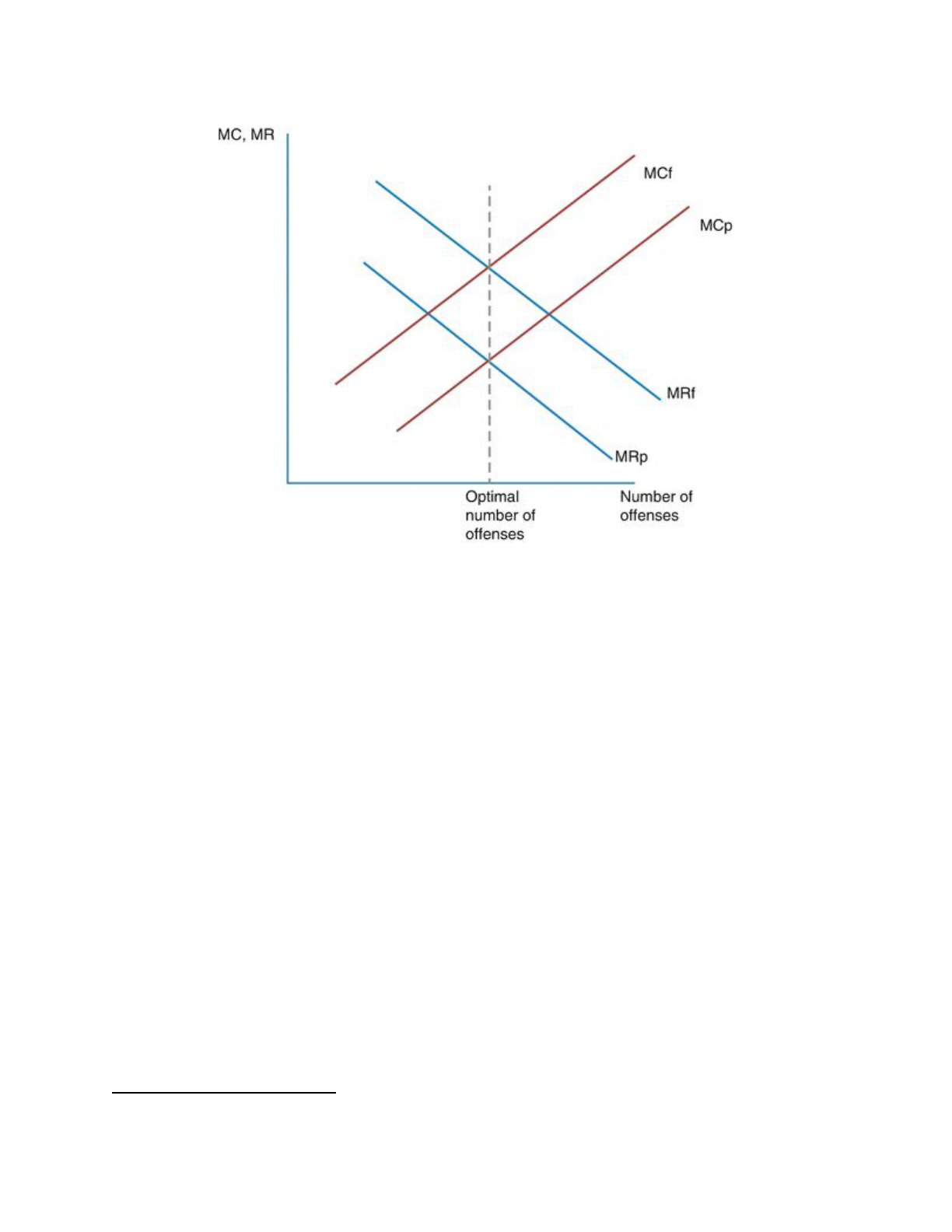
Figure 2: Becker’s Theory of Crime
2
Becker explains with the increase of the total number of offenses, the marginal cost in
committing a crime increases, while the marginal revenue for the individual decreases. F
and P
represent the cost of punishment and the probability of conviction, respectively.
It has been noted that most individuals who commit murder do not adhere to rational
decision making; yet it can be expanded to most murders under the assumption that there is
always a risk-reward approach to a perpetrator’s actions. As a result, including all murders in a
population is not inappropriate. By expanding on Becker’s theory of crime, Daniel Nagin (2012)
furthered development research on the topic by creating the following model:
RDR f(Z ) X M
it
= α
i
+ β
it
+ γ
it
+ δ
it
+ ε
it
2
https://link.springer.com/referenceworkentry/10.1007%2F978-1-4614-7883-6_17-1

Butterfield 13
The model shows that the murder rate ( ) is homicides per 100,000 residents inRDR M
it
state i
in year t
. is an expected cost function of committing a capital homicide that depends(Z )f
it
on the vector of death penalty or other sanction variables with the parameter measuring Z
it
γ
the effect of the death penalty on homicide rate. Importantly, this effect is assumed to be
homogenous across states i
and year t
.
This study applied certain economic and social modifications to examine how execution
rates affect the murder rates in the United States. Variables analyzed are first and foremost the
murder rates (per 100,000) in all fifty states, and total annual executions by year in all states.
Additionally, variables included were additional factors that could affect the outcomes, such as
unemployment rates. ( )X δ
it
I will use a panel data method similar to Nagin and Zimmerman. A primary benefit of
panel data is that one observes homicide and execution rates in the 50 states over multiple years.
This allows a researcher to effectively account for unobserved features of the state or of the time
period that might be associated with both the application of the death penalty and the homicide
rate. Some states may have different social norms or ways of thinking that could lead to a bias in
in murder rates or execution rates. The cultures in a progressive California and a more
conservative Texas are somewhat different in this regard.
The panel data accounts for these differences. , which is also referred to as the state α
i
fixed effect, allows the mean homicide rate to vary by state, while is the time fixed effect, β
it
allowing the mean homicide rate to vary over time. Finally, is the random variable that will ε
it
account for all error terms. This accounts for all the unobserved factors that determine the
homicide rate.

Butterfield 14
IV. Model Specification and Results
The empirical model used in this study is designed to examine the execution rate’s effect
on murder rates over the recent years in which some states have imposed a moratorium on the
death penalty. To properly examine the hypothesis, the state level panel data will cover the
periods of 2013-2017 for the 50 states, excluding the District of Columbia. This is to examine the
implications of the death penalty in a post-moratorium era in the country.
The econometric modeling used for the ordinary least squares and fixed effects models is
as follows:
nMU RDER lnExecution Incarcpcnt UnemRate Blackpcnt lnBachelor l
it
= β
0
+ β
1 it
+ β
2 it
+ β
3 it
+ β
4 it
+ β
5 it
+ ε
it
Where:
lnMURDER
is the dependent variable in the empirical model which measures the
murders per 100,000 residents by state by year.
lnExecution
measures all of the prisoners on death row who have been arrested,
convicted, and executed. This does not factor in any prisoners that were wrongly convicted, as
those who were executed innocently are a part of the execution statistics, and those who were let
go are not factored in. This coefficient is expected to have a negative sign since previous
findings either resulted in a negligible effect on the murder rate or a decrease in murder rate.
lnIncarc
measures the logarithm of the incarceration rate of a specific state. As
previously stated, being incarcerated is seen as a marginal cost that one associates with the risk
of committing a crime. If it is proof that incarceration is a deterrent in a rational offender’s
mindset when committing a murder, than a higher population in jail or prison may lead to an

Butterfield 15
offender’s thinking that there is a higher chance that they will not get away with their crimes,
resulting in the potential murderer not going through with the act due to the marginal cost of
them going to prison. This may be a matter of endogeneity however, and must be looked at
carefully. Consequently, the expected coefficient is expected to be negative according to
Becker’s theory of crime.
UnemRate
measures the unemployment rate percentage that comes from the number of
unemployed United States citizens divided by all that are currently in the labor force. According
to Grogger’s (1998) Model of Unemployment and Crime, as the unemployment rate goes up, the
crime rate, both violent and passive, is also expected to increase. This coefficient is expected to
have a positive effect on all of the occasions of murder.
Black
measures the percentage of African Americans in a state. This is an important
variable because it helps measure another aspect of state demographics. Past studies have found
that black males are affected by murder rates higher than white males and females. (Gender was
not included in this study because there are only a few rare exceptions when women have been
sentenced to death in the United States.) It is expected that black
is to have a positive effect on
murder rates, however the interpretation of this variable is complicated and must be taken with a
grain of salt. Zimmerman (2004) noted that race is one of the most controversial aspects of
capital punishment. In a review of numerous studies of the death penalty, the U.S. General
Accounting Office (1990) found that individuals who murdered whites were much more likely to
be sentenced to death than if their victim was non-white. I believe that this information will not
greatly affect the results of the ordinary least squares and fixed effect method, but it could affect
the interpretation of the results.

Butterfield 16
lnBachelor
measures the amount of the state population over 25 that has obtained a
bachelor’s degree. To include an education variable was critical because it measures certain
socio-demographics. Those with degrees have higher access to higher paying jobs which
theoretically incentivizes them to work in legal trades, and are generally more satisfied in their
adult lives. The variable is expected to have a negative impact, since more bachelor’s degrees
will likely result in higher quality of living, resulting in lower murder rates.
Murder rates consist of all three degrees of killing, including premeditated,
non-premeditated, (also known as a crime of passion) and manslaughter. It is important to note
that only premeditated murders are considered for the death penalty. The dependent variable in
the empirical model accounts for the total occurrences of all documented murders, with crime
data and statistics collected from the Bureau of Justice Statistics. It is important to note that these
murder rate statistics do not include all crimes that occur, but are reported and documented. This
aggregate data consists of the compilation of data collected by local law enforcement agencies
and federal law agencies.
To account for socio-demographic and state specific variables, the number of
unemployed citizens in a state, the percentage of the population over 25 with a bachelor degree,
and a proxy for race are added that accounts for a given state’s population of black citizens. All
of these variables are included in the panel data set and were sourced from the US Census
Bureau. The state specific economic variable of interest included in the study is the executions,
which was collected by the Death Penalty Information Center.
An incarceration variable was added as a deterrent variable, since it represents the
likelihood of an offender being caught and convicted. Increased incarceration rates would

Butterfield 17
theoretically have served as an increasing deterrent to commit a crime because it represents the
total marginal cost with committing a crime, rather than only the potential cost of getting caught
by an investigator or the police.
The panel data may not include all of the variables that may account for the variation in
the relationship between execution rates and murder rates since it is impossible to see all of the
variables that affect murder. This is an inherent flaw in ordinary least squares (OLS)
methodology that was originally conducted. To use all of the aspects of the panel data and
control for all of the different states and years, fixed effects were added to the state level data.
Fixed effects, a method used to assist in controlling for omitted variable bias due to unobserved
heterogeneity, are added to attempt to eliminate the variation in murders caused by factors that
vary across states but are still constant over time; also known as year-specific heterogeneity.
V. Results Interpretation
In order to determine if execution rates can affect murder rates both OLS and one-way
fixed effects models were used. In the econometric model, using an F-test to compare the
one-way fixed effect model to the OLS estimators showed that F=98.33 with p=0.0001. A
different and additional method of statistical analysis may have been able to identify a greater
estimation technique, but the results suggest that the model is improved when controlling for a
state fixed effect. I will now discuss the outcomes of the OLS estimation and controlling for the
fixed-effect.
Using OLS, I observed a 0.001 percent increase in murder rates for every 1 percent
increase in executions. However, this result was not statistically significant at a 90 percent level.

Butterfield 18
This finding changed when using the fixed effect method, strengthening to a 0.082 percent
increase in murders with the same increase in executions. The range set by standard deviations
was 0.057. At a 95 percent significance level, this is the most surprising aspect of the fixed effect
model as it relates to the variable of interest in the study. The fixed effect model found execution
rates to have a positive effect on the total rate of murders. This result is not in line with the
economic theory that an increased state execution rate results in a lower average murder rate.
There were also several other statistically significant variables in the first OLS model.
With 95 percent signifance, a one percent increase in unemployment resulted in a 0.04 percent
increase in murder rates in both the OLS and fixed effect models. Using the fixed effect model
compared to the OLS model saw no change in the significance level, with both at 95 percent.
The range set by standard deviation was 0.019. This coefficient is quite low, however, it is in line
with the theoretical framework suggesting that an increase in unemployment will increase the
amount of crime (Becker 1968).
The findings also suggest that for every one percent increase in a state’s incarceration
percentage, murders increased by 0.172 percent at a 95 percent significance level. Although once
again not in accordance with prediction and sentiment, the variable did not prove to be at a 90
percent significance level when tested with the fixed-effect method, which was to be expected
using that model.
Next, for every one percent increase in bachelor’s degrees, murder rates when tested with
the OLS method decreased by 0.088 percent. This proved to be in line with theory as murder
rates decrease with a higher education level. When testing using the fixed effects method, the
variable was found to be insignificant.

Butterfield 19
Finally, for every one percent increase in a state’s black population percentage, murders
increased by 0.031 percent. Originally tested at a 99 percent significance level with OLS, the
variable decreased in significance when tested at fixed-effect, decreasing to a 0.019 percent
increase in murders yet remaining at the 90 percent significance level. The range set by standard
deviation was 0.006. This result is in line with theory and sentiment, but as mentioned in the
variable discussion, it must be taken lightly. Black and white discrimination in the U.S. justice
system has been present for its entire history, and is likely a large determinant factor in guilty
murder convictions.
VI. Conclusion
In an effort to determine the capital punishment rate’s effect on murder rates in the
United States, the study concluded that there is not sufficient evidence that executions have some
impact on reducing murder rates, failing to satisfy my hypothesis. With improved methodology
compared to the OLS modeling, using fixed effects resulted in a 0.082 percent increase in
murders for every one percent increase in executions.
In a post-moratorium era for the death penalty, factoring in the findings, research would
suggest that prohibiting the use of capital punishment would decrease the number of murders. It
can be assumed that the use of capital punishment is near negligible, with figure 1 showing the
number of murders has decreased in the studied years compared to those previous.
In comparison to previous research, the study furthers the inconclusivity of the
homicide-punishment relationship. Dezhbakhsh (2003) found that there was a strong deterrent
effect, while Nagin (2012) and Katz (2003) found that there could be no established connection

Butterfield 20
between the two. When comparing the findings between post-moratorium years and previous
ones in the literature, the inconsistency in results continued.
There are some limitations in researching the effect of capital punishments on homicides
as a whole. The shortcomings in existing research suffer two specific flaws that make them
uninformative about the effect of capital punishment on homicide rates. First, the relevant
question regarding the deterrent effect of the death penalty is the “differential deterrent effect” of
execution compared to the detererrent effect of life imprisonment. Most convicts, regardless of
execution rates by state, are sentenced to life sentences without the possibility of parole and
never face death. None of the studies reviewed account for the severity of non-capital
punishment in their analyses. Second, the absence of the differential deterrent effect points out
the lack of study of how no capital punishment affects a potential murderer. With only the capital
punishment side being included in the studies, it presents a serious flaw of data interpretation in
the entire field of research.
For this study specifically, there were several limitations on my research. It is impossible
to capture all of the economic and intangible variables that could be a determinant of murders, so
there are likely to be several omitted variables that would benefit the model. Identifying these
variables would be beneficial in adding to the model’s explanatory power and a reduction to
omitted variable bias. Variables that could be included in future studies could account for more
socio-demographic issues, such as age groupings, income, and divorce rates. Furthermore,
locating data for more than the five years was troublesome, and more annual data would help
improve this study. Lastly, all of the aforementioned limitations in the field of study, such as
determining the proper homicide-capital punishment lag, made it difficult to analyze the research

Butterfield 21
with confidence even though many variables were statistically significant. If a different variable
could be used, a change in education would be appropriate. Using a high school diploma or an
associate degree variable would serve as a better education variable, since criminals tend to be
less educated (Lochner 2004).
It should be noted with past findings that even if executions are a deterrent to homicides,
it does not mean that capital punishment should be imposed. The sentencing of innocent inmates
to death is one of the many flaws of the United States justice system and its method of capital
punishment. Further measures must be enacted to ensure those uncommon mistakes do not
happen.

Butterfield 22
VII. References
Becker, G. S. 1968. Crime and Punishment: An Economic Approach
. Journal of Political
Economy 78, 526–536.
Dezhbakhsh, Hashem, Paul H. Rubin, and Joanna Shepherd. 2003. Does capital punishment have
a deterrent effect? New evidence from post-moratorium panel data
. American Law and
Economics Review 5:344–76.
Ehrlich, Isaac. 1975. The deterrent effect of capital punishment: A question of life and death
.
American Economic Review 65:395–417.
Grogger, Jeff. 1998. Market Wages and Youth Crime
. Journal of Labor Economics 16: 756–91.
Glaze, Lauren. “Correctional Populations in the United States, 2013.” Bureau of Justice Statistics
(BJS), 19 Dec. 2014, https://www.bjs.gov/index.cfm?ty=pbdetail&iid=5177.
Kaeble, Danielle. “Correctional Populations in the United States, 2014.” Bureau of Justice
Statistics (BJS), 29 Dec. 2015, https://www.bjs.gov/index.cfm?ty=pbdetail&iid=5519.
Kaeble, Danielle. “Correctional Populations in the United States, 2015.” Bureau of Justice
Statistics (BJS), 26 Dec. 2016, https://www.bjs.gov/index.cfm?ty=pbdetail&iid=5870.
Kaeble, Danielle. “Correctional Populations in the United States, 2016.” Bureau of Justice
Statistics (BJS), 26 Apr. 2018, www.bjs.gov/index.cfm?ty=pbdetail&iid=6226.
Katz, Lawrence, Steven D. Levitt, and Ellen Shustorovich. 2003. Prison conditions, capital
punishment, and deterrence
. American Law and Economics Review 5:318–43.
Lochner, and Moretti. “The Effect of Education on Crime: Evidence from Prison Inmates,
Arrests, and Self-Reports.” American Economic Review
, The American Economic
Association, 1 Mar. 2004, www.aeaweb.org/articles?id=10.1257/000282804322970751.

Butterfield 23
Nagin, Daniel, et al. 2012. Deterence and the Death Penalty
. National Research Council of the
National Academies 4:48-71
U.S. General Accounting Office (1990), “Death Penalty Sentencing: Research Indicates Pattern
of Racial Disparities,” report GAO-GDD-90-57.
Zimmerman, P. R. 2004. State Executions, Deterrence, and the Incidence of Murder
. Journal of
Applied Economics, 7(1), 163–93.
“Population Distribution by Race/Ethnicity.” The Henry J. Kaiser Family Foundation, 4 Dec.
2019, www.kff.org/other/state-indicator/distribution-by-raceethnicity/.

Butterfield 24
VIII. Appendix
Table 1: Variable Definitions
and Sources
Variable
Definition
Source
lnMurder
Murders per 100,000
residents by state by year
Bureau of Justice Statistics
lnBachelor
Bachelor’s degrees per
100,000 residents held by
those 25 years and older
Bureau of Labor Statistics
lnExec
Total executions by year by
state
The Death Penalty
Information Center
UnemRate
Annual average
unemployment rate by state
Bureau of Labor Statistics
blackpcnt
percent of state population
that is black
US Census Bureau
incarcpcnt
percent of state population
that is incarcerated
Bureau of Justice Statistics

Butterfield 25
Table 2: Descriptive Statistics
Variable
N
Mean
Std Dev
Min
Max
Range
Expected
Sign
MurderRate
250
4.525
2.235
0.904
12.424
11.520
Dependent
Variable
UnemRate
250
5.252
1.471
2.400
9.600
7.200
+
BachelorRate
250
33.226
6.148
21.815
50.337
28.522
-
Exec
250
0.585
2.015
0
16.000
16.000
-
blackpcnt
250
9.800
9.112
0.374
36.447
36.073
+
Incarcpcnt
250
1.873
0.737
0.759
6.245
5.486
-
Note: 50 states shown in 5 observed murder years (2013-2017). All of the descriptive statistics
are shown before taking logarithms.

Butterfield 26
Table 3: Murders
Table 3: Murders/Execution
OLS
FE
Dependent Variable
lnMurder
lnMurder
Intercept
***0.7567*** (8.03)
-0.6931 (-0.32)
Unemployment
**0.040** (2.24)
**0.040** (2.09)
lnBachelor
***-0.088*** (-3.05)
-0.093 (-0.68)
lnExec
0.001 (0.10)
**0.082** (1.43)
blackpcnt
***0.031*** (10.16)
*0.019* (3.18)
incarcpcnt
**0.172** (2.31)
0.097 (1.66)
N
250
250
R-Squared
0.5248
0.8682
F-Value
53.89
97.33
Note: t-values are in
parenthesis. *,**, and ***
denote significance at the 90
percent, 95 percent, and 99
percent level, respectively

Butterfield 27
IX. SAS Code
/** Import an XLSX file. **/
PROC IMPORT DATAFILE="/folders/myfolders/SeniorProject/FINALEXCELDRFT2.xlsx"
OUT=WORK.sp2020
DBMS=XLSX
REPLACE;
RUN;
/** Print the results. **/
PROC PRINT DATA=WORK.sp2020; RUN;
proc means data=work.sp2020;
var Population Murder Black Unemployment Bachelor Exec Incarc;
run;
/** adtnlvar = aditional variables included**/
data adtnlvar;
set work.sp2020;
/** Murder Rate is murders per 100,000 state residents**/
/** Bachelor Rate is bachelor Degrees per 100,000 state residents**/
MurderRate = Murder/(Population/100000);

Butterfield 28
BachelorRate = Bachelor/(Population/100000);
lnIncar = log(Incarc);
blackpcnt = ((Black/Population)*100);
Incarcpcnt = ((Incarc/Population)*100);
lnBachelor = log(BachelorRate);
lnMurder = log(MurderRate);
lnincarce = log(Incarcpcnt);
proc means;
var Black Unemployment BachelorRate Exec
Incarc lnMurder lnIncar lnBachelor blackpcnt Incarcpcnt MurderRate;
run;
proc means;
var MurderRate Unemployment BachelorRate Exec blackpcnt Incarcpcnt;
proc reg data=adtnlvar;
model lnMurder = Unemployment lnBachelor Exec blackpcnt lnincarce;
run;
proc reg data=adtnlvar;
model lnMurder = Unemployment lnBachelor blackpcnt lnincarce;
proc sort data=adtnlvar;
by year;
proc panel data=adtnlvar;
title fixed effect murder rates;

Butterfield 29
id state year;
model lnMurder = Unemployment lnBachelor Exec blackpcnt
lnincarce/FIXONE;
run;
